2. Download & Process Data

In this second section, we determine the north/south and east/west boundaries for your map, download data, and process it. In the next (third) section we will bring it into OpenOrienteering Mapper and make edits.
NOTE: In these instructions, the word 'mosaic', 'image' and 'template' is used interchangeably, for two reasons. Firstly, in SAGA we will create "mosaics" by joining LIDAR tiles together, then exporting them as single PNG image file. Secondly, in OpenOrienteering Mapper, when we want to load a file as an uneditable image we will load it as a "template".
2.1 Download OSM data
We will begin by determining where our map will be, and downloading the OSM data.
It is simplest to determine the rough boundary of your map at the very beginning using OpenStreetMap because you can write down the left, right, top, and bottom boundaries. It makes downloading data much easier. Additionally, if you need to expand the map later on, you can simply export a new small area outlining only the new section you want to add, rather than having to download the entirety of the larger map.
NOTE: You will need to download OSM and LIDAR data for your map. The larger these data sets, the more processing power your computer will need, and the longer it will take to process (from minutes to hours). Therefore, it is recommended to select a smaller map range for your first map. If you want to expand the map later on, it can be done and is not too much trouble.
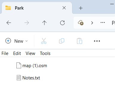
- Create a new folder on your computer and rename it the name of your map. For this example we'll call the folder "Park".
- Open https://www.openstreetmap.org.
- Zoom in on the area you want to map.
- Click the "Export" tab at top.
- Click the "Manually select a different area" link beneath the export coordinates.
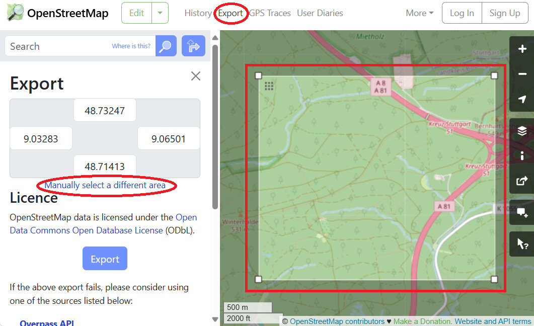
- Adjust the rectangle so that it fits the area you want to map.
- Create a new text file in the "Park" folder called "Notes.txt". Copy the top, bottom, left and right coordinates to the file, labeling it 'OSM range (degrees)'.
- OSM range (degrees): north 48.71413 to 48.73247, east 9.03283 to 9.06501
- Use the internet (i.e., https://www.latlong.net/lat-long-utm.html) to convert the south west and north east points from decimal degrees to UTM.
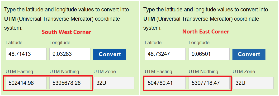
- Type the converted UTM range into the "Notes.txt" file.
- OSM range (UTM): north 5395678 to 5397718, east 502415 to 504780
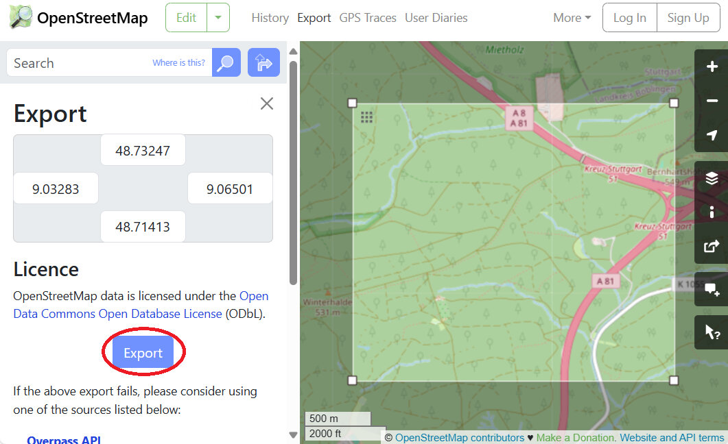
- Return to the OSM window, and click the blue "Export" button, and save the OSM file to the map folder, "Park".
NOTE: If the OSM export area is too large or contains more than 50000 data points (frequently the case when trying to download urban areas), it will produce an error message "You requested too many nodes (limit is 50000). Either request a smaller area, or use planet.osm". The best way to overcome this error message, is to export it in smaller chunks, then connect the parts later on. It helps to write down the coordinates of your intended download, because you'll have to reload the window and re-enter the dimensions to download more sections.
In the below example, we have arbitrarily divided the area into two sections, which we would download in two separate files. Just type the coordinates in the webpage and let it automatically adjust the box size - it is more accurate than using the mouse to adjust the box size.
- OSM download 1 (degrees): north 48.71413 to 48.72000, east 9.03283 to 9.06501
- OSM download 2 (degrees): north 48.72000 to 48.73247, east 9.03283 to 9.06501 - Reload the export tab if you need to download additional sections to your folder.
- You should now have one or more *.OSM files along with the Notes.txt file in a folder on your computer, named after the name of your map or "Park" in our case.
2.2 Download LIDAR data
We will download two types of LIDAR data, in no particular order:
- Digitales Oberflächenmodell (DOM) / First Return / Treetop Elevation / Digital Surface Model (DSM)
- Digitales Geländemodell (DGM) / Last Return / Ground Elevation / Digital Terrain Model (DTM)
NOTE: Some LIDAR data is stored in a 'point cloud' format, usually LAZ, LAS, or XYZ files. Other data comes in GeoTIFF (TIF) format. We will use TIF format for the bulk of these instructions because the PDF file from British Orienteering uses that format, and Baden-Württemberg data is available in that format. If the below website doesn't work for your mapping needs, visit https://www.opendem.info/opendtm_de.html to see if there are other ways to access or process free data in your area.
- Create a sub-directory in the "Park" folder, and label it "geodata".
- Open https://opengeodata.lgl-bw.de/#/ and click "zum Portal".
- Zoom in on the area you want to map.
- Scroll down and click on "Digitales Oberflächenmodell (DOM1)".
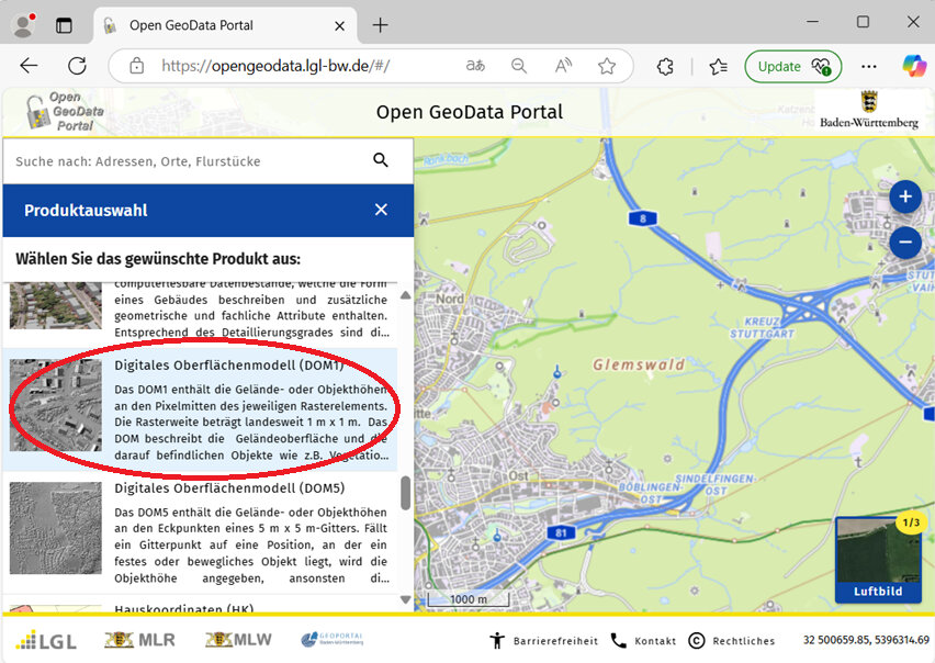
- Select which grids mark the area you intend to map.
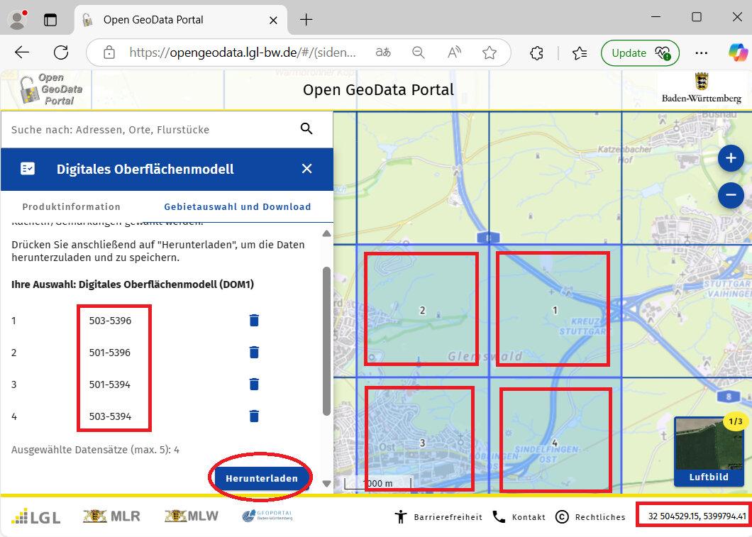
- Make a note of the filename numbers of the areas you selected. Each number represents the southwest coordinates of the area contained in each file. (The coordinates here are in UTM/meters not degrees.) The first three digits represents east/west km, and the last four digits represents north/south km. If you move the mouse over the map and look at the bottom-right of the window, it indicates the cursor location in UTM coordinates. By comparing the two, we can see that each box contains roughly four square kilometers of points (2km x 2km). For example, the file 501-5396 contains data from east 501000 to 502999, and from north 5396000 to 5397999.
- Write down the filenames (four in our example) in the "Notes.txt" file.
- DOM files: 501-5396, 501-5394, 503-5394, 503-5396
- OPTIONAL. Write down the overall range of the selected DOM data (which may be hard to do if your area is not rectangular shaped). Writing down the numbers is helpful to understand the size of the area we are downloading, and will help us to delete unnecessary files later.
- DOM range (UTM): north 5394000 to 5397999, east 501000 to 504999
- Click the "Herunterladen" button to download the files.
- Move all these zip files from downloads to the "geodata" folder.
- Right click on each zip file and select "Extract All" and extract them to that same "geodata" folder.
- Delete the zip files.
- Search for "*.tif" files in your geodata directory.
- Select all the found TIF files and "move" them to the "geodata" folder.
NOTE: Another way to go about this is to, one by one, open each decompressed folder, select all the TIF files, and cut and paste them to the "geodata" folder.
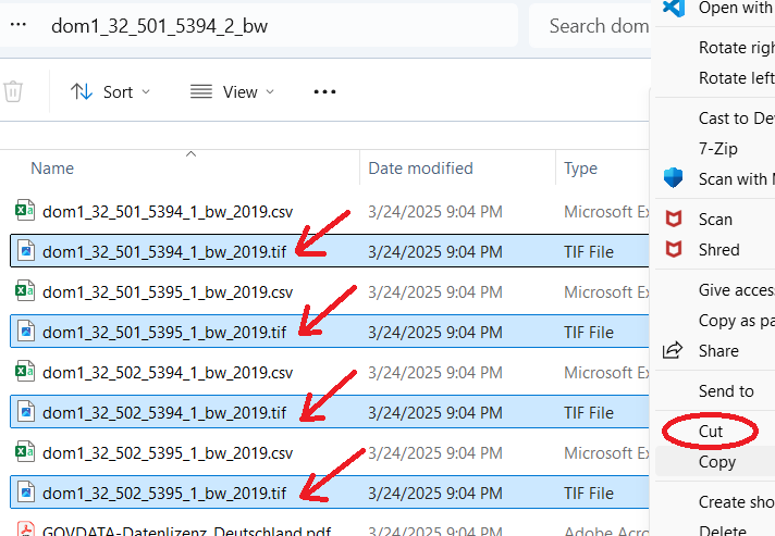
- Delete the remaining folders. All we want to keep are the TIF files.
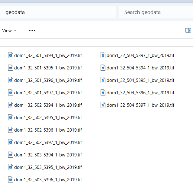
- In our example, we are left with 16 TIF files.
NOTE: By examining the filenames, we can see that each of the four zip files we downloaded earlier contained four separate files, each containing one-square-kilometer of data.
- Return to https://opengeodata.lgl-bw.de/#/.
- Zoom in on the same area we want to map.
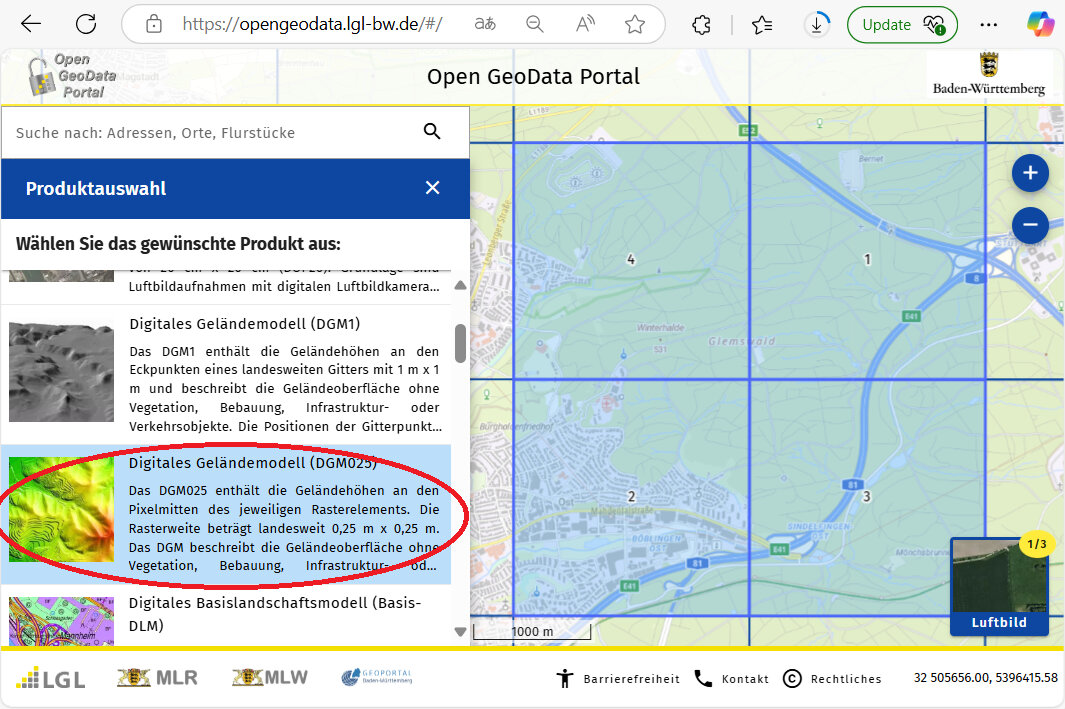
- Scroll down to and click on "Digitales Geländemodell (DGM025)".
NOTE: I would have used the DGM1 data, except those files are in XYZ format, which I would have to convert to TIF later on in order to use them in conjunction with the DOM1 files to create the vegetation_height image. Let's use the DGM025 files which are in TIF format already!
- Follow the same steps above for the DGM025 data as we did earlier for the DOM1 data. Download and extract the files, and move the TIF files to the geodata folder, removing the leftover extracted folders and anything else inside them.
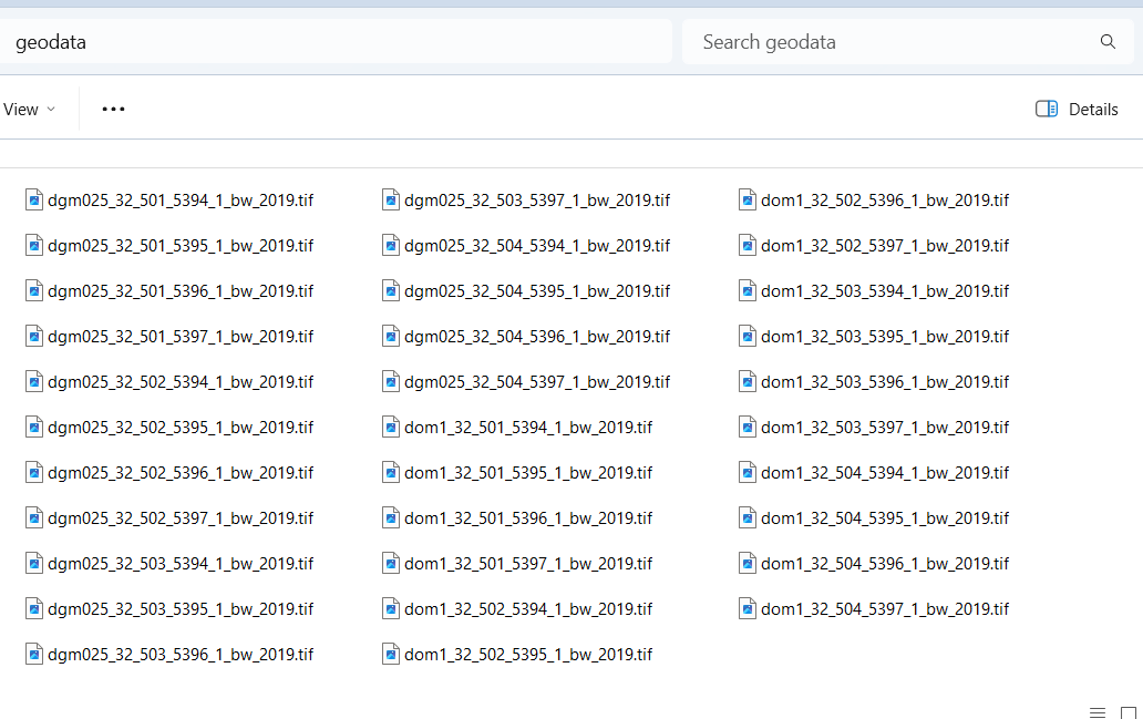
- In the geodata folder of our example, we have now 32 LIDAR files (16 DOM1 and 16 DGM025 files).
- OPTIONAL. To save processing time, we could compare the LIDAR files we've downloaded with the UTM range we wrote down earlier, and delete any files that are outside of that range. For example, we could delete the eight TIF files labeled 501-XXXX because our map only goes as west (low) as 502,415. Similarly, we could delete the eight TIF files labeled XXX-5394 because our map only goes as south (low) as 5395,678. Those together constitute 14 unnecessary files. If you are concerned about saving time and disk space, go ahead and delete any unnecessary files at this point, otherwise you can always crop your map later on. For the sake of demonstration, we will delete them.
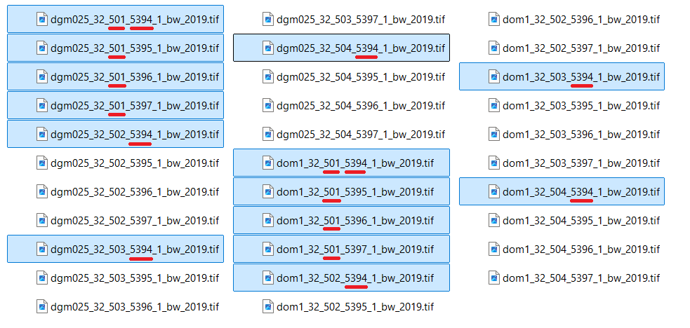
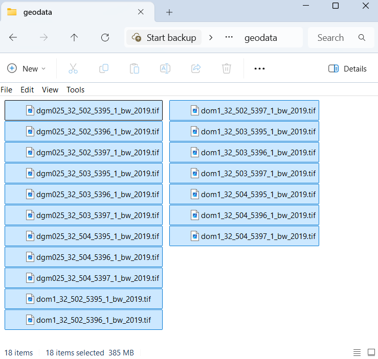
- For our demonstration, 18 LIDAR files (consuming 385MB disk size) now remain in our geodata folder.
2.3 Open LIDAR in SAGA
If you have not yet downloaded SAGA GIS, head to the link above, download it, and install it on your computer.
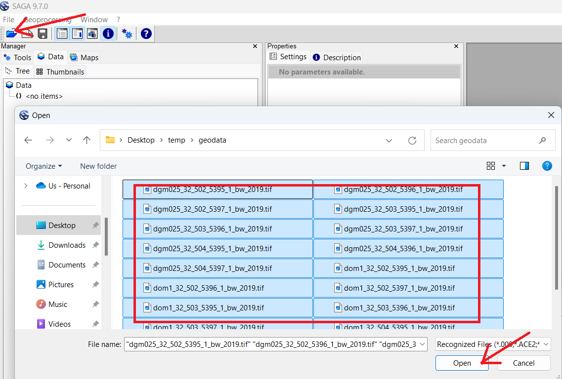
- Open the SAGA GUI program.
- Click the Folder icon or click "File->Open" to load files.
- Open the geodata folder and select all the LIDAR data.
- Click "Open".
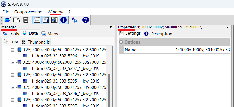
NOTE: When using SAGA, on the far left is the "Manager" window. We can see the LIDAR files we just loaded in this window, and any other files we've created. Right of that is the "Object Properties" window, which we will use to adjust properties of selected files. If either window is closed, simply select the "Window" menu, and re-check the option you wish to see.
NOTE: By "Processing" the LIDAR data, we will essentially be creating several new images and shapefiles from the LIDAR data, which we will later import or load-as-template into OpenOrienteering mapper. Once we're done creating these files, we will delete the geodata folder along with all the original LIDAR data files. If you need to pause and resume these steps later on, click on the "disk" icon or select "File-->Project-->Save as" to save the SAGA GUI working environment.
NOTE: If you make a mistake when editing the 'Object Properties' window, you may attempt to 'undo' your mistakes by clicking the 'x' in the top right of the window. Unfortunately, the changes will stay - all you accomplish by clicking the 'x' is to close the window (click 'Window' menu option to open the windows again). I have not yet figured out how to undo some changes made to the 'Object Properties'. Your best bet may be to remove whichever file you were working on, and restart the process from an earlier step. If any steps are hard to understand or cause problems, please inform the author so improvements can be made.
2.4 Altitude Elevation Mosaic
NOTE: Creating the Altitude and Treetop mosaic images essentially 'stitches' together several (smaller) LIDAR tiles into a single large tile (image). We then create several intermediate template image files from these two initial mosaics. Later on some of the processing (i.e., creating a contour shapefile) can take a very long time, and it may seem as if your computer has crashed, but let it keep running! If your computer seriously cannot handle processing the quantity of data for a large map, one alternative would be to create smaller mosaics, instead of a single large one (or even skip creating a mosaic in the first place, and use the individual tiles to create multiple altitude and treetop images). However, this strategy would require a lot more work because you would have to go through the rest of the instructions for each image file. It is recommended to go through these instructions with a smaller map first.
To create our first mosaic (image), we will use the Digitales Geländemodell (DGM) / Last Return / Ground Elevation / Digital Terrain Model (DTM) data.
- Click the gear button, also known as the "Run Tool".
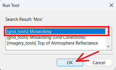
- In the "Search for" box type "mos" and press "Okay".
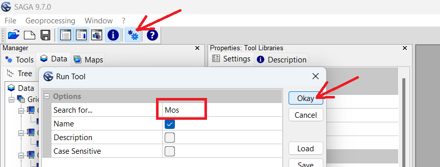
- Ensure "Mosaicking" is selected, and press "OK".
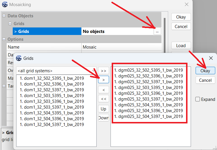
- In the Mosaicking window, click the "..." button to open the 'Grids' selection window.
- Select all the DGM025 files, then click the single ">" button to move only those files to the right.
- Click "Okay".
- Change Cellsize from 0.25 to 1.
- Change Fit from Nodes to "cells".
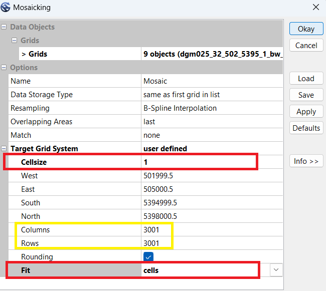
- Examine the quantity of columns and rows. In this example we see 3001. These numbers will have to exactly match the dimensions when we create the Treetop Elevation Mosaic in the next step.
- Write the dimensions in the Notes.txt file.
- DGM Mosaic: columns 3001, rows 3001
- Click "Okay". Wait for the process to complete.
- Single-click the new "Mosaic" file at the bottom of the left-hand Manager window.
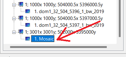
- In the Object Properties window, change the Name to "Altitude".
- Press Enter twice to 'apply' the change.
- Scroll to the bottom of the Object Properties window, at Colors and select the "..." button.
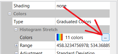
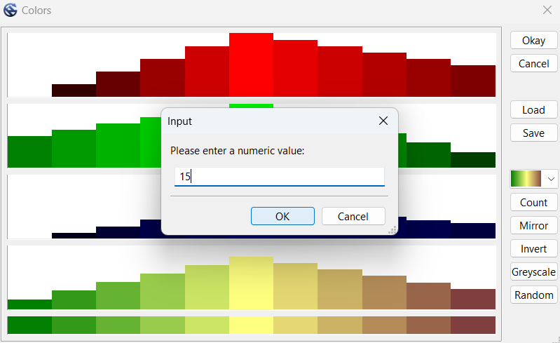
- Click the color button and change it to the 11th option up from the bottom (green-yellow-brown).
- Click "Count" button, and change it to 15.
- Click "Okay" to close the Colors window.
- In the Object Properties window, click "Apply" to apply changes.
NOTE: Although we could press the 'Save' button, all it would do is offer to save the current configuration into an external file for reloading. We will use a different function 'Save as Image' to export an image file for our map.
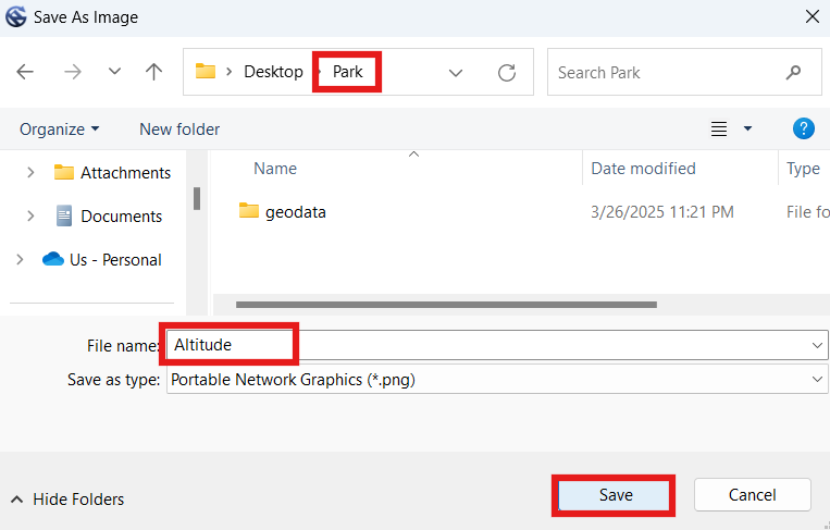
- In the Manager window, right-click the "Altitude" file and select "Save as Image".
- Label the image "Altitude".
- Select your "Park" folder (not the geodata folder), and click "Save".
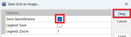
- Ensure "Save Georeference" is checked. "Legend" can remain un-checked.
- Click "Okay".
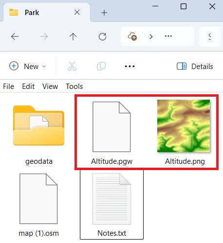
- You should now have an Altitude image (PNG) and world file (PGW) in your Park folder.
2.5 Treetop Elevation Mosaic
For our second mosaic (image), we will use the Digitales Oberflächenmodell (DOM) / First Return / Treetop Elevation / Digital Surface Model (DSM) data.
- Click the gear button.
- In the "Search for" box type "mos" and press "Okay".
- Ensure "Mosaicking" is selected, and press "OK".
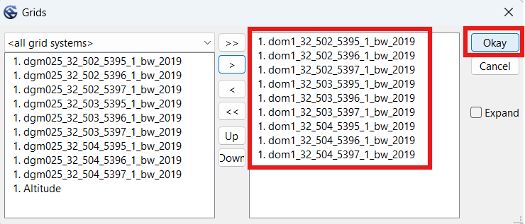
- In the Mosaicking window, click the "..." button to open the 'Grids' selection window.
- Click the double "<<" button to move all the files to the left-hand side.
- Select all the DOM1 files this time, then click the single ">" button to move only those files to the right.
- Click "Okay".
- Set Cellsize to 1.
- Set Fit to "cells".
- Compare the quantity of columns and rows with the previous DGM mosaic (Altitude) we entered in our notes. Mine first showed 3000 but I was able to get it to show 3001 by switching Fit to "nodes" and back to "cells" again. If that does not work for you, go ahead and edit the numbers. Alternatively, you could change the Target Grid System to "grid or grid system", then select the "Altitude" option. However you do it, the dimensions will have to be the same as Altitude, for a later step. In our example, we need the dimensions to be 3001 x 3001.
NOTE: Do not press the 'default' button, because it will clear the north, south, east and west values. To reload the ones that were there before, you may have to load the Mosaicking function again, switch up the source elements, or restart the instructions from an earlier step.
- Click "Okay". Wait for the process to complete.
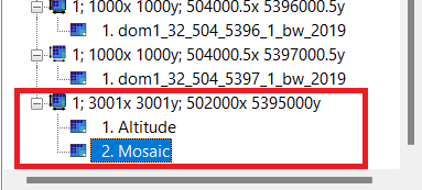
NOTE: Both Altitude and Mosaic must be under the same line listing the dimensions. If both mosaics are not under the same dimensions, delete/close one or both Mosaic files, and redo previous steps until you are able to get their dimensions to match.
- Click the new "Mosaic" file.
- In the Object Properties window, change the Name to "Treetops".
- Press Enter twice to 'apply' the change.
- Scroll to the bottom of the Object Properties window, at Colors and select the "..." button.
- Click the color button and change it to the 11th option up from the bottom (green-yellow-brown).
- Click "Count" button, and change it to 15.
- Click "Okay" to close the Colors window.
- In the Object Properties window, click "Apply" to apply changes.
NOTE: Although we could press the 'Save' button, all it would do is offer to save the current configuration into an external file for reloading. We will use a different function 'Save as Image' to export an image file for our map.
- In the Manager window, right-click the "Treetops" file and select "Save as Image".
- Label the image "Treetops".
- Select the base directory of your map (Park folder), and click "Save".
- Check the "Save Georeference" box. "Legend" can remain un-checked.
- Click "Okay".
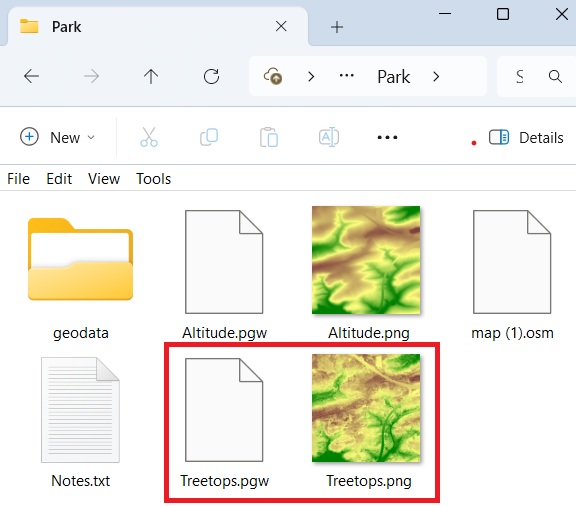
- You should now have Altitude and Treetops images (PNG) and world files (PGW) in your Park folder.
2.6 Vegetation Height Image
We will use the difference between the other two mosaics to create a third image.
- Examine the bottom of the Manager window (on the left hand side of the SAGA GUI window). We should see both mosaics underneath the same dimensions grid, in our example they are both underneath "1; 3001x3001y; 502000x 5395000y". Because they are both underneath that line, we are good to proceed. If the two mosaics appear under different dimension lines, we will need to re-create one or both mosaics, so that both appear under the same size dimensions.
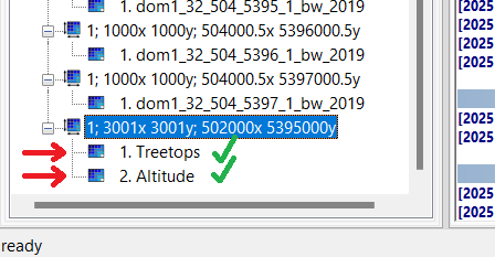
- Click the gear button.
- In the "Search for" box type "dif" and press "Okay".
- Select "Grid Difference", and press "OK".
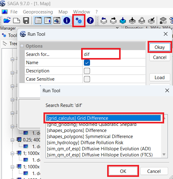
- In the Grid Difference window, in "Grid System" select the dimensions which both mosaics are under. In our example, we've selected "1; 3001x3001y; 502000x 5395000y".
- Under "> > Minuend", select "Altitude".
- Under "> Subtrahend", select "Treetops".
- Under "< < Difference", select "create".
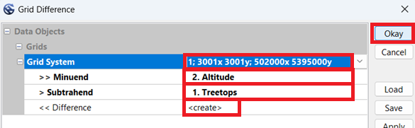
- Click "Okay". Wait for the process to complete.
- Click the new "Difference" file at the bottom of the left-hand Manager window.
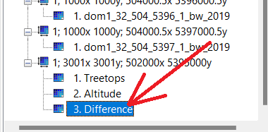
- In the Object Properties window, change the Name to "Vegetation_Height".
- Press Enter twice to 'apply' the change.
- Scroll down in the Object Properties window, until you get to the Display section.
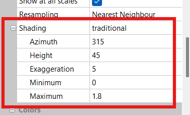
- Change Shading from "none" to "traditional".
- Set Azimuth to "315".
- Set Height to "45".
- Set Exaggeration to "5".
- Set Minimum to "0".
- Set Maximum to "1.8".
- Scroll to the bottom of the Object Properties window.
- Set Colors --> Type to "Graduated Colors".
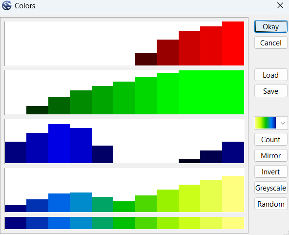
- Under Colors and select the "..." button.
- Click the color button and change it to the 2nd option up from the bottom (yellow-green-blue).
- Click "Count" button, and change it to 11.
- Click the "Mirror" button.
- Click "Okay" to close the Colors window.
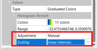
- Set Adjustment to "Manual"
- Set Scaling to "linear intervals".
- In the Object Properties window, click "Apply" to apply changes.
NOTE: Although we could press the 'Save' button, all it would do is offer to save the current configuration into an external file for reloading. We will use a different function 'Save as Image' to export an image file for our map.
- In the Manager window, right-click the "Vegetation_Height" file and select "Save as Image".
- Label the image "Vegetation_Height".
- Select the base directory of your map (Park folder), and click "Save".
- Check the "Save Georeference" box. "Legend" can remain un-checked.
- Click "Okay".
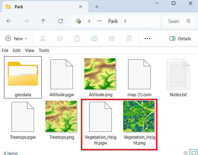
- You should now have a third image (PNG) file named "Vegetation_Height" and world files (PGW) in your Park folder.
2.7 Vegetation Slope Image
We will create another image calculated from the slopes in the vegetation height mosaic.
- Click the gear button.
- In the "Search for" box type "slope" and press "Okay".
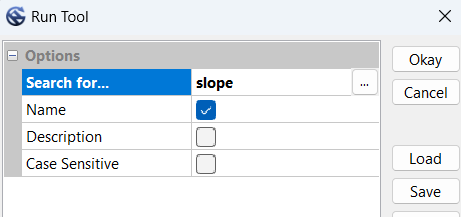
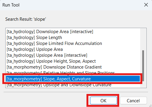
- Select "Slope, Aspect, Curvature", and press "OK".
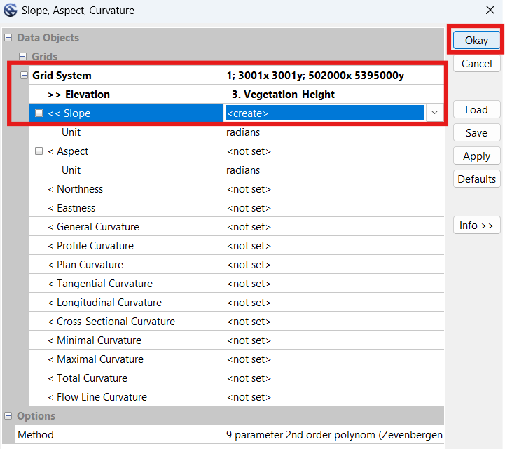
- In the Slope, Aspect, Curvature window, in "Grid System" select the dimensions which both mosaics are under. In our example, we've selected "1; 3001x3001y; 502000x 5395000y".
- Under "> > Elevation", select "Vegetation_Height".
- Under "< < Slope", select "create".
- Click "Okay". Wait for the process to complete.
- Click the new "Slope" file at the bottom of the left-hand Manager window.
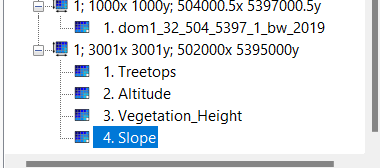
- In the Object Properties window, change the Name to "Vegetation_Slope".
- Press Enter twice to 'apply' the change.
- Scroll to the bottom of the Object Properties window.
- Set Colors --> Type to "Graduated Colors".
- Under Colors and select the "..." button.
- Click the color button and change it to the 2nd option up from the bottom (yellow-green-blue).
- Click "Count" button, and change it to 11.
- Click the "Mirror" button.
- Click "Okay" to close the Colors window.
- Scroll to the bottom of the Object Properties window.
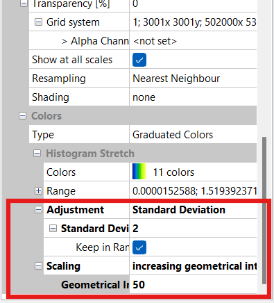
- Change Adjustment from "none" to "Standard Deviation".
- Set Standard Deviation to "2".
- Set Keep in Range to "enabled".
- Set Scaling to "increasing geometric intervals".
- Set Geometric Intervals to "50".
- Click "Apply".
NOTE: Although we could press the 'Save' button, all it would do is offer to save the current configuration into an external file for reloading. We will use a different function 'Save as Image' to export an image file for our map.
- In the Manager window, right-click the "Vegetation_Slope" file and select "Save as Image".
- Label the image "Vegetation_Slope".
- Select the base directory of your map (Park folder), and click "Save".
- Check the "Save Georeference" box. "Legend" can remain un-checked.
- Click "Okay".
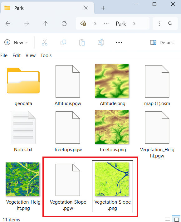
- You should now have a fourth image (PNG) file named "Vegetation_Slope" and world files (PGW) in your Park folder.
2.8 Raw 0.5m Shapefile
We will now create a shape file containing raw (not simplified) contours for the area at 0.5m interval. The shape file we produce will not be directly imported into Open Orienteering mapper, but rather used to create a micro-contour template-image, because being able to view micro contours is really useful when mapping. In this step we will only create the intermediary shape file containing the contours.
- Click the gear button.
- In the "Search for" box type "contour" and press "Okay".
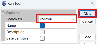
- Ensure "Contour Lines from Grid" is selected, and press "OK".
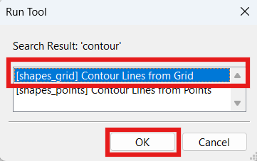
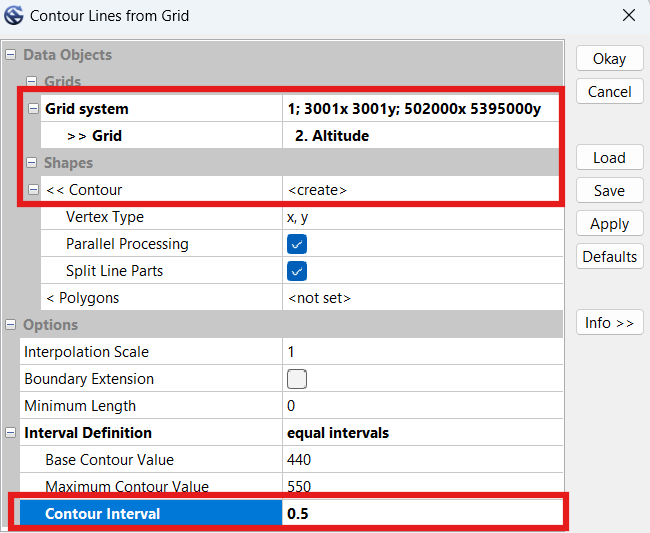
- In the Contour Lines from Grid window, in "Grid System" select the dimensions which the earlier mosaics are under. In our example, we've selected "1; 3001x3001y; 502000x 5395000y".
- Under "> > Grid", select "Altitude".
- Under "< < Contour", select "create".
NOTE: Here the SAGA program will automatically select the 'Base Contour Value' and the 'Maximum Contour Value' for us. The values shown in the screenshot below only apply to my example area.
- Under "Contour Interval", select "0.5".
- Click "Okay".
- Your computer may take a while to complete this task. My computer took 100 seconds to complete it for the example area, but for a larger area it took the same computer over 30 minutes to finish the process.
NOTE: Although we could press the 'Save' button, all it would do is offer to save the current configuration into an external file for reloading. We will use a different function 'Save as...' to export an ESRI Shape File for our map.
- In the Manager window, scroll to the bottom and right-click on the new Shape file "Altitude [Interval 0.5]" file and select "Save as...".
- Label the output file "Contours_0.5m_Raw.shp".
- Select the base directory of your map (Park folder), and click "Save".
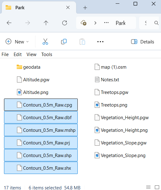
- You should now have six additional files saved to your Park folder.
2.9 Smooth 2.5m Shapefile
We will now run a simplify function twice to smooth elevation data, then use that data to create smoothed (simplified) contour lines for the map at 0.5m interval.
- Click the gear button.
- In the "Search for" box type "simple" and press "Okay".
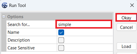
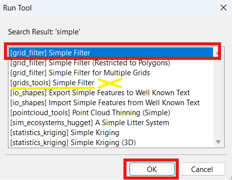
- Ensure "[grid_filter] Simple Filter" is selected, and press "OK".
- In the Simple Filter window, in "Grid System" select the dimensions which the earlier mosaics are under. In our exaple, we've selected "1; 3001x3001y; 502000x 5395000y".
- Under "> > Grid", select "Altitude".
NOTE: There are two "Simple Filter" functions. If you accidentally ran the wrong function, named "[grids_tools] Simple Filter", it will not offer any options here because it is looking for a 'Grid Collection' instead of a 'Grid'. If this is the case, close the function and run the correct function, "[grid_filter] Simple Filter".
- Under "< Filtered Grid", select "create".
- Under "Radius", select "5".
NOTE: For less hilly areas, try 10 here instead of 5.
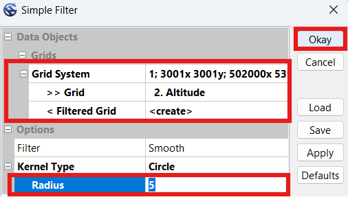
- Click "Okay". Wait for the process to complete.
- Click the new "Altitude [Smoothed]" file at the bottom of the 'Grids' files in the left-hand Manager window.
- In the Object Properties window, change the Name to "Altitude_Smoothed_5m" (or whichever radius value you used for the first time).
- Press Enter twice to 'apply' the change.
NOTE: In steps 11-20 we will repeat some of the above steps to create a second simplified image, based off the first simplified image. If you experiment and find that doing it a second time does not help, please skip to step 24 and proceed with only one file.
- Click the gear button.
- In the "Search for" box type "simple" and press "Okay".
- Again, select "[grid_filter] Simple Filter", and press "OK".
- In the Simple Filter window, in "Grid System" select the dimensions which the earlier mosaics are under. In our exaple, we've selected "1; 3001x3001y; 502000x 5395000y".
- Under "> > Grid", select the previously created smoothed file. In our case it was called "Altitude_Smoothed_5m".
NOTE: If it won't let you select anything for Grid, you may have run the wrong 'Simple Filter' function. Close the function and re-run the "[grid_filter] Simple Filter" function (step 14).
- Under "< Filtered Grid", select "create".
- Under "Radius", select "1" or "2".
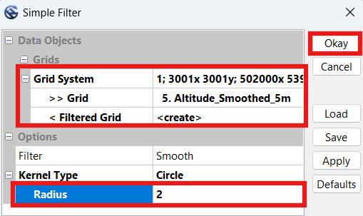
- Click "Okay". Wait for the process to complete.
- Click the new "Altitude_Smoothed_5m [Smoothed]" file at the bottom of the 'Grids' files in the left-hand Manager window.
- In the Object Properties window, change the Name to "Altitude_Smoothed_5m_2m", to indicate the smoothing was first to 5m, and then to 2m (or whichever radius value you used for the second time).
- Press Enter twice to 'apply' the change.
NOTE: We will not be saving either of these files to image files, but instead use them to create contour shape files. The purpose of smoothing the file twice at different levels is to reduce contour line jagginess. You may try experimenting with different values instead of 5-2 to see which values offer the best balance between accuracy and smoothness for your map.
- We should now have two smoothed grid files at the bottom of the 'Grid' section of the left-hand Manager window.
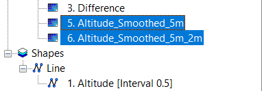
- Click the gear button.
- In the "Search for" box type "contour" and press "Okay".
- Ensure "Contour Lines from Grid" is selected, and press "OK".
- In the Contour Lines from Grid window, in "Grid System" select the dimensions which the earlier mosaics are under. In our example, we've selected "1; 3001x3001y; 502000x 5395000y".
- Under "> > Grid", select "Altitude_Smoothed_5m_2m", or whatever you named it in step 20.
- Under "< < Contour", select "create".
NOTE: Here the SAGA program will automatically select the 'Base Contour Value' and the 'Maximum Contour Value' for us. The values shown in the screenshot below only apply to my example area.
- Under "Contour Interval", enter "2.5" or whichever contour interval you want on your map.
NOTE: If you're using a value other than 2.5m, it may help to experiment with different radius values in the simple filter functions earlier in this section to see if they work better for your map.
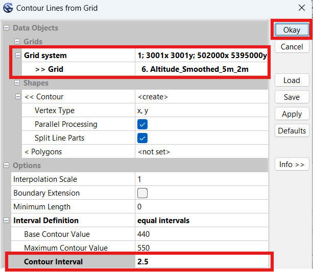
- Click "Okay".
- Wait a short while before the computer finishes this task. My computer took under 30 seconds.
NOTE: Although we could press the 'Save' button, all it would do is offer to save the current configuration into an external file for reloading. We will use a different function 'Save as...' to export an ESRI Shape File for our map.
- In the Manager window, scroll to the bottom and right-click on the new Shape file "Altitude_Smoothed_5m_2m [Interval 2.5]" file and select "Save as...".
- Label the output file "Contours_2.5m_Smooth.shp".
- Select the base directory of your map (Park folder), and click "Save".
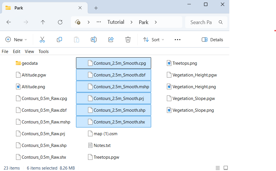
- You should now have six additional files saved to your Park folder.
2.10 Blue & Black Slope Images
- Click the gear button.
- In the "Search for" box type "curv" and press "Okay".
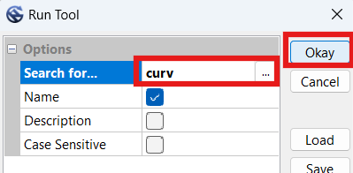
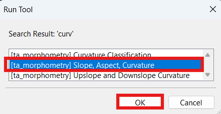
- Ensure "Slope, Aspect, Curvature" is selected, and press "OK".
- In the Simple Filter window, in "Grid System" select the dimensions which the earlier mosaics are under. In our exaple, we've selected "1; 3001x3001y; 502000x 5395000y".
- Under "> > Elevation", select "Altitude".
- Under "< < Slope", select "create".
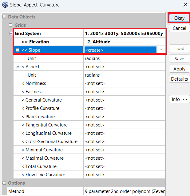
- Click "Okay". Wait for the process to complete.
- Click the new "Slope" file at the bottom of the 'Grids' files in the left-hand Manager window.
- Scroll down in the Object Properties window, until you get to the Display section.
- Change Shading from "none" to "traditional".
- Set Exaggeration to "150".
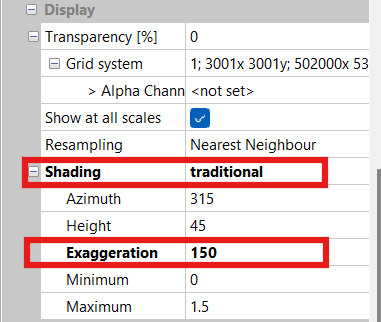
- Scroll to the bottom of the Object Properties window.
- Set Colors --> Type to " RGB Compsite".
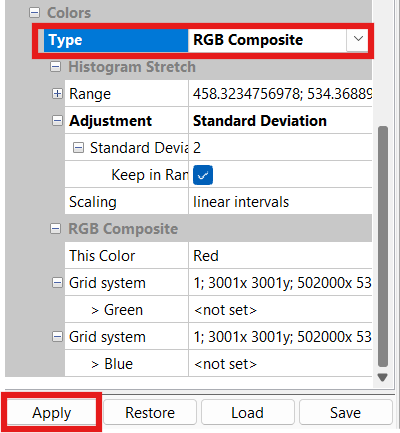
NOTE: It will automatically populate the values in the Range box; no changes required.
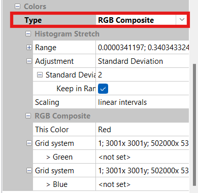
- Click "Apply".
NOTE: Although we could press the 'Save' button, all it would do is offer to save the current configuration into an external file for reloading. We will use a different function 'Save as Image' to export an image file for our map.
- In the Manager window, right-click the "Slope_Blue" file and select "Save as Image".
- Label the image "Slope_Blue".
- Select the base directory of your map (Park folder), and click "Save".
- Check the "Save Georeference" box. "Legend" can remain un-checked.
- Click "Okay".
- Go to the bottom of the Object Properties window, to the Display section.
- Change Colors --> Type from "RGB Composite" to "Shade".
- Change Adjustment --> Standard Deviation to "5".
NOTE: It will automatically populate the values in the Range box to reflect the change; no adjustments are required to these numbers.
- Change Scaling to "increasing geometrical intervals".
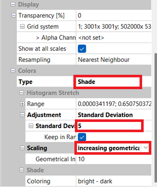
- Click "Apply".
NOTE: Although we could press the 'Save' button, all it would do is offer to save the current configuration into an external file for reloading. We will use a different function 'Save as Image' to export an image file for our map.
- In the Manager window, right-click the "Slope_Gray" file and select "Save as Image".
- Label the image "Slope_Gray".
- Select the base directory of your map (Park folder), and click "Save".
- Check the "Save Georeference" box. "Legend" can remain un-checked.
- Click "Okay".
- You should now have slope images (PNG) named "Slope_Blue" and "Slope_Gray" and corresponding world files (PGW) in your Park folder.
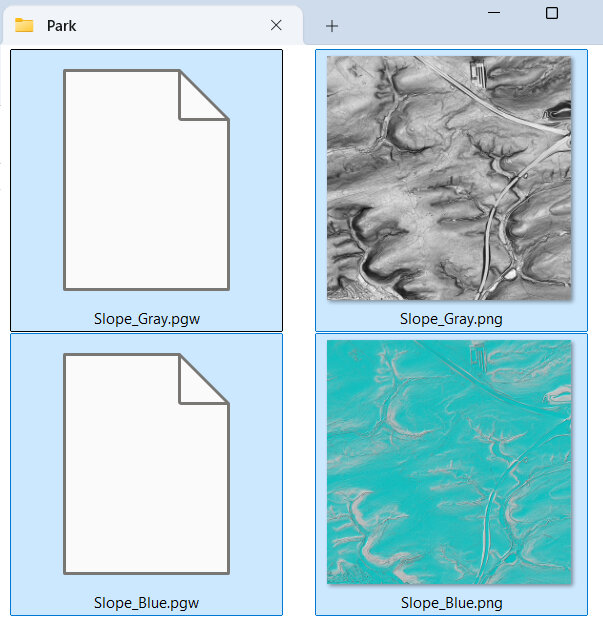
2.11 Blue Hill-Shading Images
For this step we will use the original 'Altitude' mosaic from earlier in this tutorial to create some blue hill-shading images.
- Select the Altitude file in the Manager window.
- In the Object Properties window, scroll down to the 'Colors' section. It should show green-yellow-brown and 15 colors from the original 'Altitude' image. This setting means that the final product should turn 'blue', which is what we want. If your colors are not adjusted properly, return to this step and fix them before proceeding, or the end result will not be blue but other colors.
- Scroll up to "Shading", and change it from "none" to "Traditional".
- Set Azimuth to "315".
NOTE: Azimuth is the direction of the imaginary light source/sun, NW in this case. The image we create will best highlight features running perpendicular to this angle.
- Set Height to "45".
NOTE: Height is the virtual sun’s altitude. It may be worth experimenting with altering the “Max” value a little.
- Set Exaggeration to "50".
NOTE: Exaggeration values between 50 and 150 work best. It’s a balance between under-shading small features such as ditches and earthbanks and over-shading hillsides. Higher values work better in flatter areas.
- Set Minimum to "0".
- Set Maximum to "1.5".
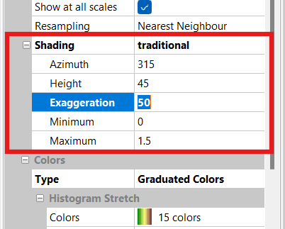
- Scroll down to "Colors" and change "Type" to "RGB Composite".
NOTE: Although we could press the 'Save' button, all it would do is offer to save the current configuration into an external file for reloading. We will use a different function 'Save as Image' to export an image file for our map.
- In the Manager window, right-click the "Altitude" file and select "Save as Image".
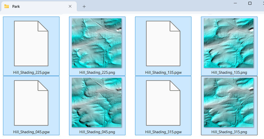
- Label the image "Hill_Shading_315" (for the azimuth setting in the Shading option).
- Select the base directory of your map (Park folder), and click "Save".
- Check the "Save Georeference" box. "Legend" can remain un-checked.
- Click "Okay" to save the image
- Change the Object Properties --> Shading --> "Azimuth" to "45".
- Press Enter twice to 'apply' the change.
- In the Manager window, right-click the "Altitude" file and select "Save as Image".
- Label the image "Hill_Shading_045", and click "Okay" to save the image.
- Repeat the last three steps for Azimuths "135" and "225", saving the files as "Hill_Shading_135.png" and "Hill_Shading_225.png" respectively.
- You should now have four new image (PNG) files named "Hill_Shading_XXX" with world files (PGW) in your Park folder.
2.12 Further SAGA Processing
We are done with SAGA. Close the SAGA program. If you choose to save the file, save it to the geodata folder.
Although additional steps could be taken if we had access to additional types of LIDAR data, this guide does not explain how to:
- Process intermediate-return (point cloud) LIDAR into different classifications of undergrowth (i.e., thick vegetation vs light vegetation).
- Process intensity of first return for indication of type of object (i.e., tree vs building).
For further explanation on the above topics, read "Chapter 6 Obtaining a LiDAR undergrowth template using LAStools and SAGA-GIS" at this link. You may also need to obtain additional LIDAR point cloud data with intermediate returns (not just first or lasts returns). These files may not be free yet, like the open data we have already accessed. Additionally, you may need to use other programs to help process it (LASTools, or Karttapullautin).
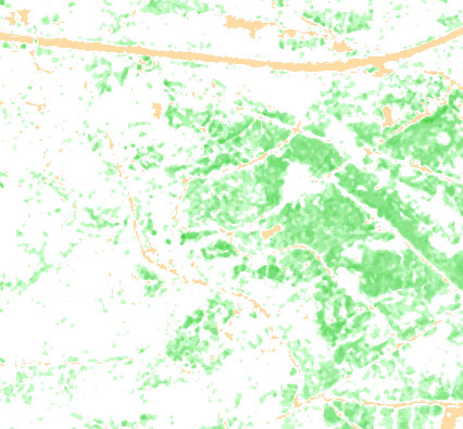
If you are able to download comprehensive LIDAR point cloud data with intermediate returns, it is super useful. As an example, you could create an image that shows how dense the vegetation is, across the entire mapped area. The downside of this sort of data, is that it may be out of season, or a few years old, and it depends upon when they conducted the last aerial survey. Below is an example of one such final product, this one was processed using Karttapullautin program, and shows different levels of undergrowth as an orienteeing map does. Such data allows the mapper to characterize the vegetation and undergrowth easily and automatically, without having to conduct extensive field mapping, or at least provides us with a great starting point for later field-checking. Imagine how cool this image would look once we load our contour lines, and open street map data!
2.13 Orthophotography
OPTIONAL STEP
Because of the way it’s surveyed, LIDAR data is usually more accurately geo-referenced than standard aerial photography.
That being said, sometimes aerial photography is invaluable when trying to draw features on your map that only exist or were observed in aerial photography. Orthophotography is special photography usable in mapping programs like OpenOrienteering Mapper, which has been adjusted to fit to normalized geo-projections.
If you have enough disk space and/or haven't used orthophotography before, you should download orthophotography that corresponds to the area you intend to map and see if it helps. A word of caution though, they are large files! It may make more sense, and save memory, to download them only when you're ready to use them, and delete them afterwards. For the sake of demonstration, we will download the files here.
- Go to the Open GeoData portal and scroll down to 'Digitales Orthophoto', select the area you want, and download it.
- Once you extract all the folders, search for TIF and TGW files (may need to do in two separate steps).
- Move all the TIF (image file) along with the TGW (world file) to a separate 'Park/Orthophotography' folder for later loading into the map (as image/template).
NOTE: I recommend placing the orthophotography files into their own sub-folder, so we don't accidentally copy them to our mobile device later when we prepare to conduct field mapping. I haven't found them all that useful when field-mapping, but your experiences may differ.
- When you are ready to use them, visit this section to load them in OpenOrienteering mapper.
2.14 Micro-Contour Template
We will now create an OpenOrienteering template using the 0.5m raw contours. If you have not yet downloaded OpenOrienteering Mapper yet, head to the link above, download it, and install it on your computer.
- Run OpenOrienteering Mapper.
- Click "Create a new map".
- Select "ISOM 2017-2_10000".
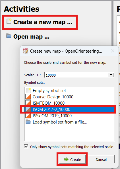
- Click "Create".
NOTE: The left-hand side of OpenOrienteering Mapper allows you to edit your map (it is grayed out until we add data). The right-hand side shows the "Symbol" window for adding objects to your map. Along the top is a toolbar that lets you select what action you want to do, adding, editing, rotating, cropping, etc. For additional help consult the online documentation page.
NOTE: In OpenOrienteering Mapper, there are two different ways to load intermediate data files: (1) loading an image file for viewing/comparing with the map, and (2) importing a (certain type of) file allowing you to edit the symbols as you would an orienteering map. For this step we will 'import' the 0.5m raw contour shape file. More on this important distinction later.
- Click "File --> Import".
- Select the "Contours_0.5m_Raw.shp" file in your Park folder.
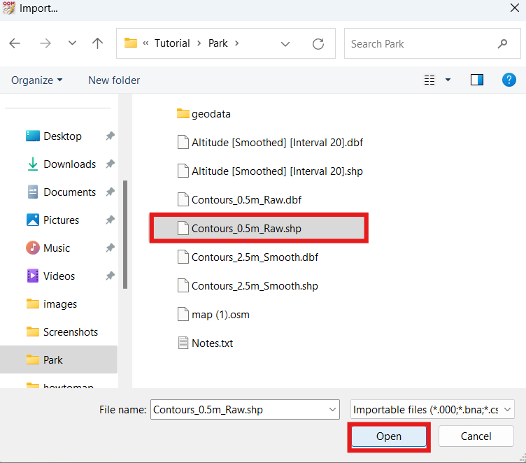
- Click "Open". Wait for it to finish loading the file.
- On the "Map Georeferencing" window, under "Coordinate reference system", select "UTM".
- Check that the "Status" indicates "Valid". If there is an error with the coordinate reference system, you may need to re-process the LIDAR correctly.
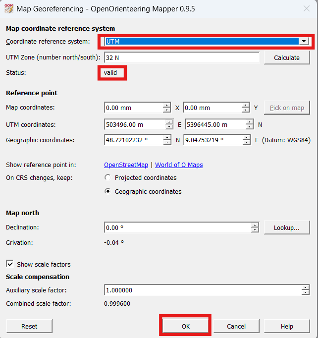
- Click "OK". Wait for it to finish thinking.
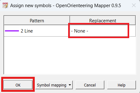
- On the "Assign new symbols" window, under the "2 Line", leave it reading "- none -", and click "OK".
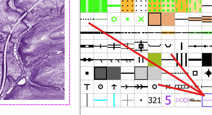
- You should now see before you a bunch of purple contour lines. At the bottom of the symbol window, double-click on the purple 2 Line symbol.
- In the "Symbol settings" window, under the "Line settings tab, change the "Line width from "0.10 mm" to "0.01 mm".
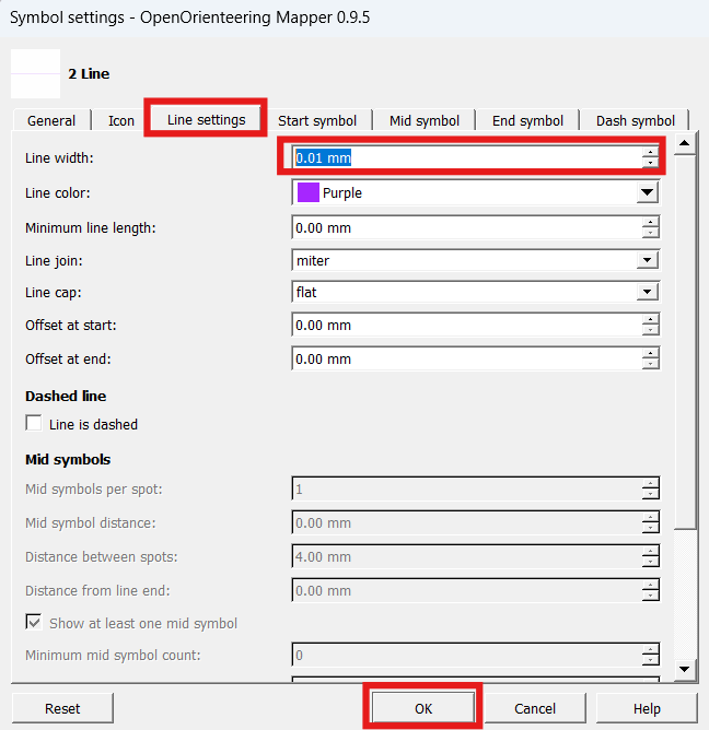
- Click "OK".
- The purple lines may appear to have disappeared, but they're still there. They're just very small, you have to zoom in to see them.
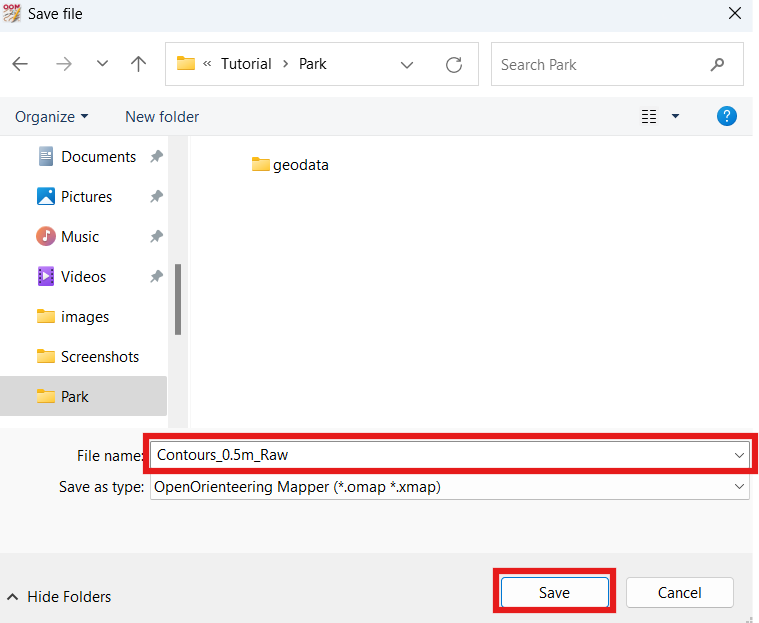
- Select File --> "Save".
- Navigate to your Park folder save the file as "Contours_0.5m_Raw.omap"
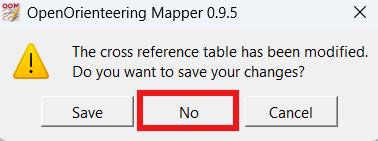
- Close the OpenOrienteering Mapper window by clicking the X at the top right of the window.
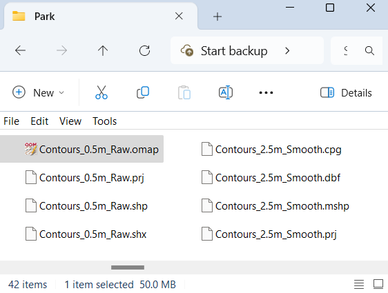
- You should now have an OpenOrienteering Mapper file in your Park folder called "Contours_0.5m_Raw.omap".